Example forecast hub data

library(hubExamples)
library(hubVis)
library(dplyr)
#> 
#> Attaching package: 'dplyr'
#> The following objects are masked from 'package:stats':
#> 
#>     filter, lag
#> The following objects are masked from 'package:base':
#> 
#>     intersect, setdiff, setequal, union
library(ggplot2)

Overview

The hubExamples package provides three data sets that contain example model output and target data for an example forecast hub: forecast_outputs, forecast_target_ts, and forecast_target_observations. These forecasts and target data are a subset of the model outputs and target data that are provided in the example-complex-forecast-hub. These data were in turn derived from forecast submissions and target data for the FluSight Forecast Hub for the 2022/23 season.

We begin with a high level overview of these data objects and then we describe the different forecast targets in more detail.

Example forecast output data

The example forecasts provided in forecast_outputs are derived from forecasts that were submitted to the FluSight hub from three models: Flusight-baseline, MOBS-GLEAM_FLUH, and PSI-DICE. The original forecasts submitted to the hub were in quantile format, but we have modified those submissions to provide examples of additional model output types and targets. The predictions for these other output types should be viewed only as illustrations of the data formats, not as real examples of forecasts. We will describe the methods used for creating other forecast output types below.

The snippet below shows the format of the forecast_outputs (note: here and throughout the document, you may need to scroll to the right within displays of code output to see all data frame columns).

head(forecast_outputs)
#> # A tibble: 6 × 9
#>   model_id          reference_date target          horizon location target_end_date output_type output_type_id value
#>   <chr>             <date>         <chr>             <int> <chr>    <date>          <chr>       <chr>          <dbl>
#> 1 Flusight-baseline 2022-11-19     wk inc flu hosp       0 25       2022-11-19      quantile    0.05              22
#> 2 Flusight-baseline 2022-11-19     wk inc flu hosp       0 25       2022-11-19      quantile    0.1               31
#> 3 Flusight-baseline 2022-11-19     wk inc flu hosp       0 25       2022-11-19      quantile    0.25              45
#> 4 Flusight-baseline 2022-11-19     wk inc flu hosp       0 25       2022-11-19      quantile    0.5               51
#> 5 Flusight-baseline 2022-11-19     wk inc flu hosp       0 25       2022-11-19      quantile    0.75              57
#> 6 Flusight-baseline 2022-11-19     wk inc flu hosp       0 25       2022-11-19      quantile    0.9               71

This is a data frame with four groups of columns (see the hubverse documentation for more information about these data formats):

The model_id identifies the model that produced the predictions.
Together, the location, reference_date, horizon, target_end_date, and target columns are referred to as “task id variables” because they serve to identify a prediction task:
- The location column contains a FIPS code identifying the location being predicted.
- The reference_date is a date in ISO format that gives the Saturday ending the week the predictions were generated.
- The horizon gives the difference between the reference_date and the target date of the forecasts (target_end_date, see next item) in units of weeks. Informally, this describes “how far ahead” the predictions are targeting.
- The target_end_date is a date in ISO format that gives the Saturday ending the week being predicted. For example, if the target_end_date is "2022-12-17", predictions are for a quantity relating to influenza activity in the week from Sunday, December 11, 2022 through Saturday, December 17, 2022.
- The target describes the target quantity for the prediction. In the above example, the target of "wk flu hosp rate" is the weekly rate of hospital admissions per 100,000 population. The targets included in this example will be described in other sections below.
The output_type and output_type_id columns provide metadata about the model predictions.
- The output_type specifies the representation of the predictive distribution.
- The output_type_id gives additional identifying information about the predictions; the information in this column is specific to the output_type.
The value column contains the value of the model’s prediction.

The original hub submissions contained predictions for many locations and dates, and quantile forecasts were provided at 23 different quantile levels ranging from 0.01 to 0.99. To make the example data more manageable, the forecast_outputs object contains a subset of these outputs for two locations (Massachusetts, FIPS code "25", and Texas, FIPS code "48") and two reference dates (2022-11-19 and 2022-12-17). Additionally, for the quantile forecasts we have subset to seven quantile levels: 0.05, 0.1, 0.25, 0.5, 0.75, 0.9, and 0.95.

The task id variables used and values of those variables are specific to each modeling hub. For example, a hub collecting predictions for locations other than US states would use a different location identifier than FIPS codes, and a hub might introduce additional task id variables such as an identifier of age group or disease variant depending on the goals of the hub. See the hubverse documentation for further information about task id variables.

Example forecast target data

All predictions are for targets that are based on influenza hospital admissions as reported in the US National Healthcare Safety Network (NHSN). The forecast_target_ts object contains the observed values of these hospital admissions in a time series format:

head(forecast_target_ts)
#> # A tibble: 6 × 3
#>   date       location observation
#>   <date>     <chr>          <dbl>
#> 1 2020-01-11 01                 0
#> 2 2020-01-11 15                 0
#> 3 2020-01-11 18                 0
#> 4 2020-01-11 27                 0
#> 5 2020-01-11 30                 0
#> 6 2020-01-11 37                 0
tail(forecast_target_ts)
#> # A tibble: 6 × 3
#>   date       location observation
#>   <date>     <chr>          <dbl>
#> 1 2023-11-11 51                88
#> 2 2023-11-11 50                 3
#> 3 2023-11-11 53                20
#> 4 2023-11-11 55                19
#> 5 2023-11-11 54                12
#> 6 2023-11-11 56                 7

The forecast_target_observations object contains the observed values for the prediction targets:

head(forecast_target_observations)
#> # A tibble: 6 × 6
#>   location target_end_date target          output_type output_type_id observation
#>   <chr>    <date>          <chr>           <chr>       <chr>                <dbl>
#> 1 US       2022-10-22      wk inc flu hosp quantile    NA                    2380
#> 2 01       2022-10-22      wk inc flu hosp quantile    NA                     141
#> 3 02       2022-10-22      wk inc flu hosp quantile    NA                       3
#> 4 04       2022-10-22      wk inc flu hosp quantile    NA                      22
#> 5 05       2022-10-22      wk inc flu hosp quantile    NA                      50
#> 6 06       2022-10-22      wk inc flu hosp quantile    NA                     124

This data frame has a subset of the columns in the forecast_outputs that is sufficient to identify the observed value corresponding to each prediction, including the location, target_end_date, target, output_type, and output_type_id, along with the observed target values, recorded in the observation column. Note that the reference_date and horizon columns are not needed in this data frame, since the target_end_date is sufficient to align observations with predictions.

Further detail on the forecast targets

The example forecast data contains the following combinations of target and output_type:

forecast_outputs |>
  distinct(target, output_type) |>
  arrange(target, output_type)
#> # A tibble: 6 × 2
#>   target                    output_type
#>   <chr>                     <chr>      
#> 1 wk flu hosp rate          cdf        
#> 2 wk flu hosp rate category pmf        
#> 3 wk inc flu hosp           mean       
#> 4 wk inc flu hosp           median     
#> 5 wk inc flu hosp           quantile   
#> 6 wk inc flu hosp           sample

We will describe each of these targets in the following sections.

The `wk inc flu hosp` target

The wk inc flu hosp target represents weekly new hospital admissions with a confirmed influenza diagnosis. We have predictions of this target with four output types: mean, median, quantile and sample. Note that the quantile predictions were contributed directly by modelers to the FluSight hub, and median predictions correspond exactly to the quantile predictions at probability level 0.5. We have obtained sample predictions from the quantile forecasts using the distfromq package by estimating the full quantile function from the submitted quantile predictions for each individual location and target date, drawing samples from those marginal distributions using the probability integral transform method, and using a copula corresponding to a discrete-time AR(0.9) Gaussian process to induce dependence across sequential horizons. Mean predictions are obtained as the mean of samples drawn for each location and target date combination.

The following plot shows the quantile and median predictions along with the observed hospital admission counts for Massachusetts and Texas.

plot_step_ahead_model_output(
  model_output_data = forecast_outputs |>
    filter(output_type %in% c("quantile", "median")),
  target_data = forecast_target_ts |>
    filter(location %in% c("25", "48"),
           date >= "2022-10-01", date <= "2023-04-01"),
  use_median_as_point = TRUE,
  x_col_name = "target_end_date",
  intervals = c(0.5, 0.8, 0.9),
  facet = "location",
  group = "reference_date",
  interactive = FALSE
)
#> Warning: ! `output_type_id` column must be a numeric. C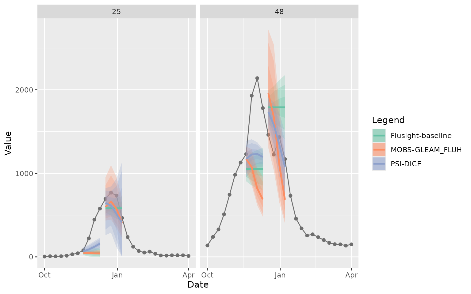lass applied by default.

The following plot shows the target data and predictive samples for just predictions for Massachusetts with reference date December 17, 2022 generated by the “MOBS-GLEAM_FLUH” model.

ggplot() +
  geom_line(
    data = forecast_target_ts |>
      filter(location == "25",
             date >= "2022-10-01", date <= "2023-04-01"),
    mapping = aes(x = date, y = observation)
  ) +
  geom_line(
    data = forecast_outputs |>
      filter(
        location == "25",
        model_id == "MOBS-GLEAM_FLUH",
        reference_date == "2022-12-17",
        output_type == "sample"
      ),
    mapping = aes(x = target_end_date, y = value, group = output_type_id),
    color = "blue",
    alpha = 0.3
  ) +
  theme_bw()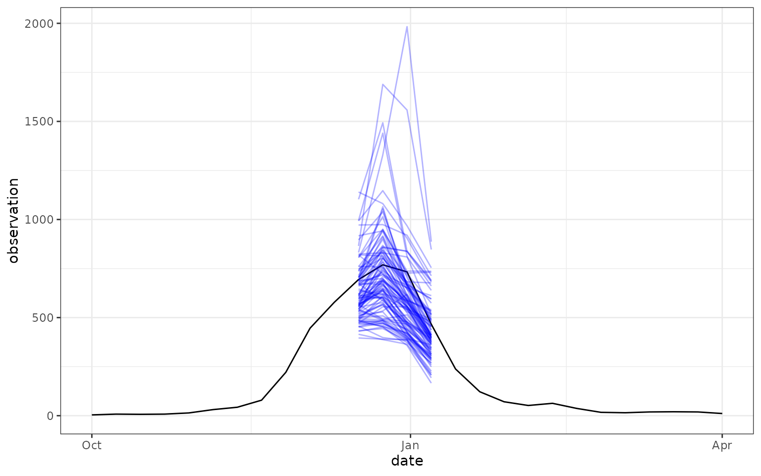

For purposes of evaluating predictions, it can be helpful to join the observed target values, contained in forecast_target_observations, into the data frame of forecast outputs. This enables direct comparison of predictions and observations. We illustrate this here, omitting some columns from the display for convenience:

forecast_outputs |>
  filter(target == "wk inc flu hosp") |>
  left_join(forecast_target_observations) |>
  select(-model_id, -reference_date, -horizon)
#> Joining with `by = join_by(target, location, target_end_date, output_type, output_type_id)`
#> # A tibble: 5,232 × 7
#>    target          location target_end_date output_type output_type_id value observation
#>    <chr>           <chr>    <date>          <chr>       <chr>          <dbl>       <dbl>
#>  1 wk inc flu hosp 25       2022-11-19      quantile    0.05              22          NA
#>  2 wk inc flu hosp 25       2022-11-19      quantile    0.1               31          NA
#>  3 wk inc flu hosp 25       2022-11-19      quantile    0.25              45          NA
#>  4 wk inc flu hosp 25       2022-11-19      quantile    0.5               51          NA
#>  5 wk inc flu hosp 25       2022-11-19      quantile    0.75              57          NA
#>  6 wk inc flu hosp 25       2022-11-19      quantile    0.9               71          NA
#>  7 wk inc flu hosp 25       2022-11-19      quantile    0.95              80          NA
#>  8 wk inc flu hosp 25       2022-11-26      quantile    0.05               5          NA
#>  9 wk inc flu hosp 25       2022-11-26      quantile    0.1               21          NA
#> 10 wk inc flu hosp 25       2022-11-26      quantile    0.25              38          NA
#> # ℹ 5,222 more rows

The `wk flu hosp rate` target

The wk flu hosp rate target represents the rate of weekly confirmed influenza hospital admissions per 100,000 population. Note that this target was not included in the FluSight hub; we have introduced it here for illustrative purposes. We have used population values of 6,978,662 for Massachusetts and 29,914,599 for Texas. These population values are sourced from the auxiliary data file provided by the FluSight hub, which are also reproduced in the example-complex-forecast-hub repository.

For this target, we created cumulative distribution function (CDF) predictions with evenly spaced CDF evaluation points ranging from 0.25 to 25 in increments of 0.25 hospitalizations per 100,000 population:

forecast_outputs |>
  filter(target == "wk flu hosp rate") |>
  select(-model_id, -reference_date, -horizon) |>
  head()
#> # A tibble: 6 × 6
#>   target           location target_end_date output_type output_type_id  value
#>   <chr>            <chr>    <date>          <chr>       <chr>           <dbl>
#> 1 wk flu hosp rate 25       2022-11-19      cdf         0.25           0.0409
#> 2 wk flu hosp rate 25       2022-11-19      cdf         0.5            0.131 
#> 3 wk flu hosp rate 25       2022-11-19      cdf         0.75           0.568 
#> 4 wk flu hosp rate 25       2022-11-19      cdf         1              0.891 
#> 5 wk flu hosp rate 25       2022-11-19      cdf         1.25           0.965 
#> 6 wk flu hosp rate 25       2022-11-19      cdf         1.5            0.985

For the CDF output_type, the output_type_id contains the value at which the predictive CDF was evaluated, and the value contains the predicted probability that the target is less than or equal to that evaluation point. In the above example, the value in the row with output_type_id equal to 1.5 contains the model’s estimated probability that the rate of hospital admissions in Texas the week of December 17, 2022 would be less than or equal to 1.5 admissions per 100,000 population. Again, these CDF values were estimated from the original quantile forecasts using the methods in the distfromq package.

The following plot illustrates the predictive CDFs produced by the MOBS-GLEAM_FLUH model for Massachusetts on the reference date 2022-12-17, with each target_end_date shown in a separate facet. Also shown in orange is a CDF representing the observation for this target, which was between 9.75 and 10 hospitalizations per 100,000 population. This CDF corresponds to a point mass at the observed value, with a value of 0 below the observation and a value of 1 above the observation.

# Subset the forecasts and observations to those that we will plot
forecasts_to_plot <- forecast_outputs |>
  filter(
    model_id == "MOBS-GLEAM_FLUH",
    target == "wk flu hosp rate",
    location == "25",
    reference_date == "2022-12-17"
  ) |>
  mutate(output_type_id = as.numeric(output_type_id))
head(forecasts_to_plot)
#> # A tibble: 6 × 9
#>   model_id        reference_date target           horizon location target_end_date output_type output_type_id    value
#>   <chr>           <date>         <chr>              <int> <chr>    <date>          <chr>                <dbl>    <dbl>
#> 1 MOBS-GLEAM_FLUH 2022-12-17     wk flu hosp rate       0 25       2022-12-17      cdf                   0.25 8.52e-21
#> 2 MOBS-GLEAM_FLUH 2022-12-17     wk flu hosp rate       0 25       2022-12-17      cdf                   0.5  1.63e-19
#> 3 MOBS-GLEAM_FLUH 2022-12-17     wk flu hosp rate       0 25       2022-12-17      cdf                   0.75 2.80e-18
#> 4 MOBS-GLEAM_FLUH 2022-12-17     wk flu hosp rate       0 25       2022-12-17      cdf                   1    4.37e-17
#> 5 MOBS-GLEAM_FLUH 2022-12-17     wk flu hosp rate       0 25       2022-12-17      cdf                   1.25 6.17e-16
#> 6 MOBS-GLEAM_FLUH 2022-12-17     wk flu hosp rate       0 25       2022-12-17      cdf                   1.5  7.87e-15

target_observations_to_plot <- forecast_target_observations |>
  filter(
    target == "wk flu hosp rate",
    location == "25",
    target_end_date %in% forecasts_to_plot$target_end_date
  ) |>
  mutate(output_type_id = as.numeric(output_type_id))
head(target_observations_to_plot)
#> # A tibble: 6 × 6
#>   location target_end_date target           output_type output_type_id observation
#>   <chr>    <date>          <chr>            <chr>                <dbl>       <dbl>
#> 1 25       2022-12-17      wk flu hosp rate cdf                   0.25           0
#> 2 25       2022-12-17      wk flu hosp rate cdf                   0.5            0
#> 3 25       2022-12-17      wk flu hosp rate cdf                   0.75           0
#> 4 25       2022-12-17      wk flu hosp rate cdf                   1              0
#> 5 25       2022-12-17      wk flu hosp rate cdf                   1.25           0
#> 6 25       2022-12-17      wk flu hosp rate cdf                   1.5            0

# We illustrate that the cdf values recorded in forecast_target_observations
# correspond to a point mass at the observed hospitalization rate.
first_one_ind <- min(which(target_observations_to_plot$observation == 1))
target_observations_to_plot[(first_one_ind - 2):(first_one_ind + 2), ]
#> # A tibble: 5 × 6
#>   location target_end_date target           output_type output_type_id observation
#>   <chr>    <date>          <chr>            <chr>                <dbl>       <dbl>
#> 1 25       2022-12-17      wk flu hosp rate cdf                   9.5            0
#> 2 25       2022-12-17      wk flu hosp rate cdf                   9.75           0
#> 3 25       2022-12-17      wk flu hosp rate cdf                  10              1
#> 4 25       2022-12-17      wk flu hosp rate cdf                  10.2            1
#> 5 25       2022-12-17      wk flu hosp rate cdf                  10.5            1

# Make the plot
ggplot() +
  geom_line(
    mapping = aes(x = output_type_id, y = value,
                  color = "forecast", linetype = "forecast"),
    data = forecasts_to_plot
  ) +
  geom_line(
    mapping = aes(x = output_type_id, y = observation,
                  color = "observation", linetype = "observation"),
    data = target_observations_to_plot,
  ) +
  scale_color_manual(
    "CDF",
    values = c("black", "orange")
  ) +
  scale_linetype_manual(
    "CDF",
    values = c(1, 2)
  ) +
  facet_wrap(vars(target_end_date)) +
  xlab("output_type_id (units are hospital admissions per 100,000 population)") +
  ylab("CDF value (units are probability)")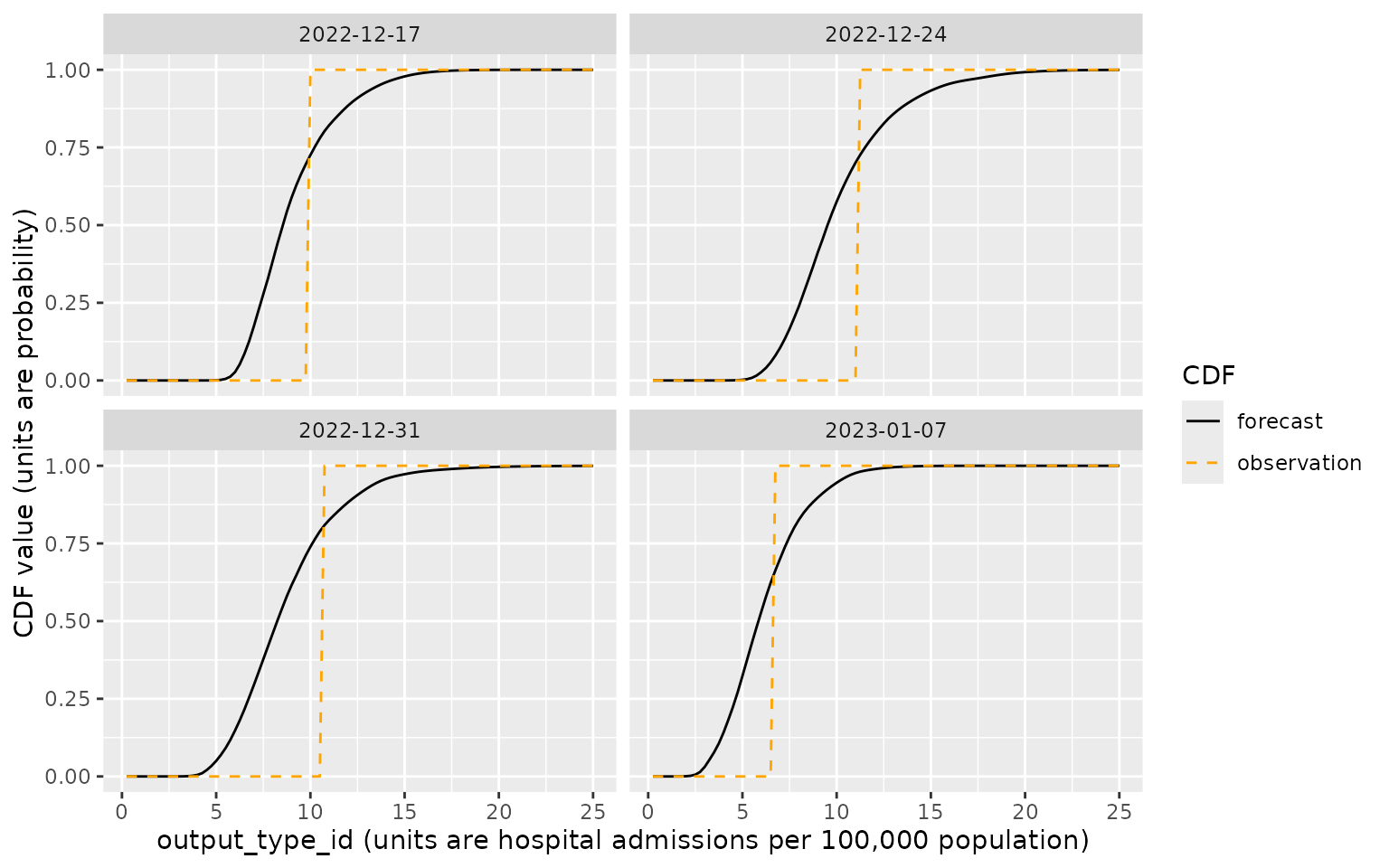

The `wk flu hosp rate category` target

The “wk flu hosp rate category” target represents a categorical intensity level of influenza activity, defined as “low” (hospital admissions rate per 100,000 $\leq$ 2.5), “moderate” (2.5 < admissions rate $\leq$ 5), “high” (5 < admissions rate $\leq$ 7.5), or “very high” (7.5 < admissions rate). The forecast_outputs object has example forecasts for this target in a PMF format, with a probability assigned to each intensity category. Again, forecasts of this target were not collected by the FluSight hub; we have derived predictions from the submitted quantile forecasts using the distfromq package. For context, the following plot displays the observed data for the 2022/23 season on the scale of hospital admissions per 100,000 population, with the boundaries of the intensity categories denoted with horizontal lines:

# a data frame containing location FIPS codes and population values
# in units of 100,000 people
population_values <- data.frame(
  location = c("25", "48"),
  population_100k = c(6978662, 29914599) / 100000
)

# compute observed hospital admission rates for the 2022/23 season
observed_rates <- forecast_target_ts |>
  filter(location %in% c("25", "48"),
         date >= "2022-10-01", date <= "2023-04-01") |>
  left_join(population_values) |>
  mutate(rate = observation / population_100k)
#> Joining with `by = join_by(location)`

# plot along with intensity thresholds
ggplot() +
  geom_line(
    mapping = aes(x = date, y = rate),
    data = observed_rates
  ) +
  geom_hline(
    mapping = aes(yintercept = y),
    linetype = 2,
    data = data.frame(y = c(2.5, 5, 7.5))
  ) +
  facet_wrap(vars(location))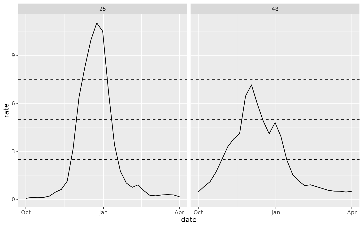

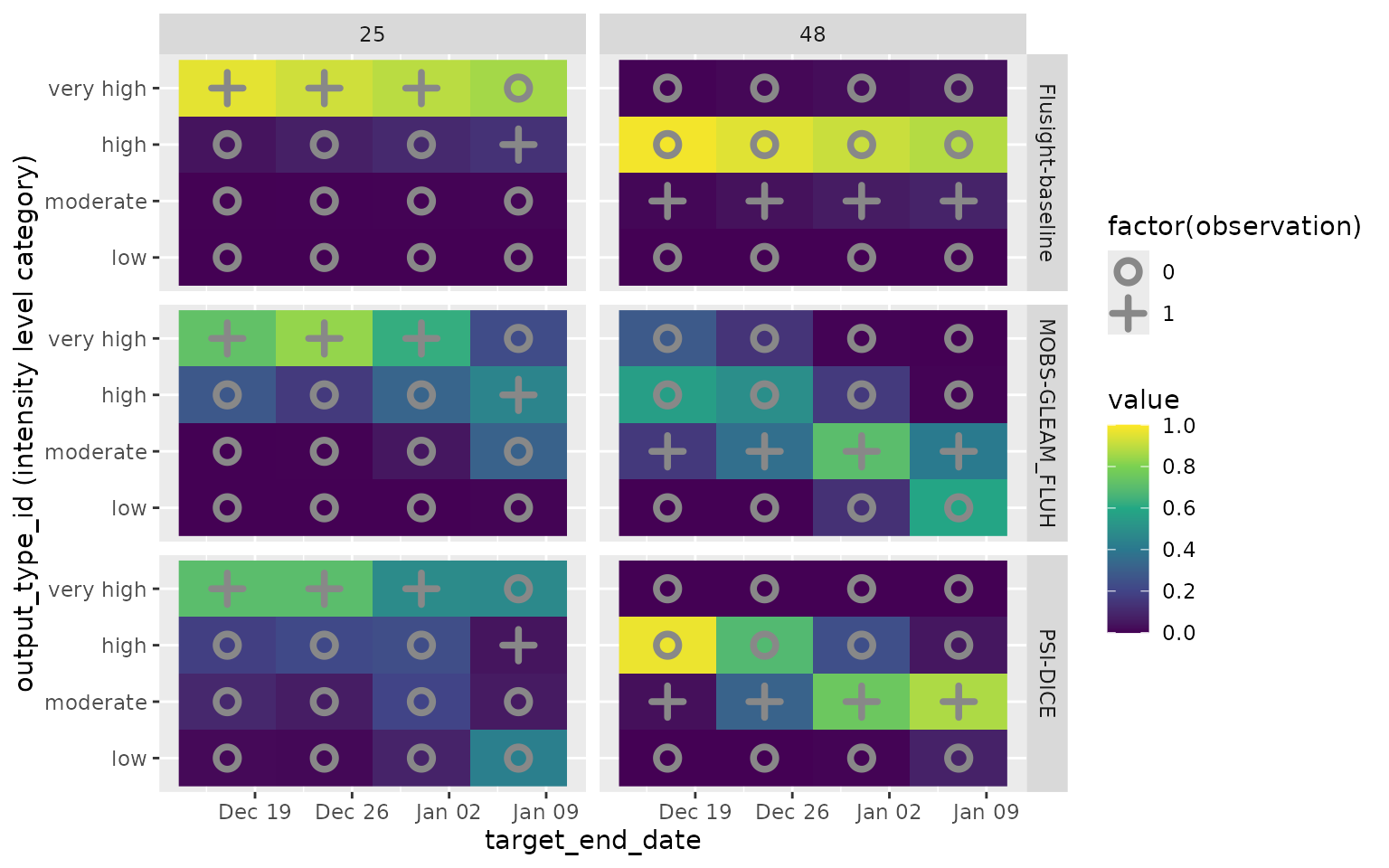
Here is a plot showing the predictive distributions for these targets from the three included models. Color indicates the predicted probability for each intensity category. The observed category is indicated with a + in the plot, while unobserved categories are indicated with an o. Here, the PMF value recorded in forecast_target_observations corresponds to a point mass at the observed category, with a value of 1 for the observed category and a value of 0 for the other categories.

# extract a subset of forecasts to plot and
# set the output_type_id to be an ordered factor
forecasts_to_plot <- forecast_outputs |>
  filter(
    target == "wk flu hosp rate category",
    reference_date == "2022-12-17"
  ) |>
  mutate(
    output_type_id = factor(output_type_id,
                            levels = c("low", "moderate", "high", "very high"),
                            ordered = TRUE)
  )
forecasts_to_plot |>
  select(-model_id, -reference_date, -horizon) |>
  head()
#> # A tibble: 6 × 6
#>   target                    location target_end_date output_type output_type_id      value
#>   <chr>                     <chr>    <date>          <chr>       <ord>               <dbl>
#> 1 wk flu hosp rate category 25       2022-12-17      pmf         low            0.0000180 
#> 2 wk flu hosp rate category 25       2022-12-17      pmf         moderate       0.00157   
#> 3 wk flu hosp rate category 25       2022-12-17      pmf         high           0.0397    
#> 4 wk flu hosp rate category 25       2022-12-17      pmf         very high      0.959     
#> 5 wk flu hosp rate category 25       2022-12-24      pmf         low            0.00000970
#> 6 wk flu hosp rate category 25       2022-12-24      pmf         moderate       0.00294

# extract the corresponding observations
observations_to_plot <- forecast_target_observations |>
  filter(
    location %in% c("25", "48"),
    target == "wk flu hosp rate category",
    target_end_date %in% forecasts_to_plot$target_end_date
  ) |>
  mutate(
    output_type_id = factor(output_type_id,
                            levels = c("low", "moderate", "high", "very high"),
                            ordered = TRUE)
  )
observations_to_plot |>
  head()
#> # A tibble: 6 × 6
#>   location target_end_date target                    output_type output_type_id observation
#>   <chr>    <date>          <chr>                     <chr>       <ord>                <dbl>
#> 1 25       2022-12-17      wk flu hosp rate category pmf         low                      0
#> 2 25       2022-12-17      wk flu hosp rate category pmf         moderate                 0
#> 3 25       2022-12-17      wk flu hosp rate category pmf         high                     0
#> 4 25       2022-12-17      wk flu hosp rate category pmf         very high                1
#> 5 48       2022-12-17      wk flu hosp rate category pmf         low                      0
#> 6 48       2022-12-17      wk flu hosp rate category pmf         moderate                 1

# plot the predictions and observations
ggplot() +
  geom_raster(
    mapping = aes(x = target_end_date, y = output_type_id, fill = value),
    data = forecasts_to_plot
  ) +
  scale_fill_viridis_c(
    breaks = seq(from = 0, to = 1, by = 0.2),
    limits = c(0, 1)
  ) +
  geom_point(
    mapping = aes(x = target_end_date, y = output_type_id,
                  shape = factor(observation)),
    color = "#888888",
    size = 3, stroke = 2,
    data = observations_to_plot,
  ) +
  scale_shape_manual(
    values = c(1, 3),
    breaks = c(0, 1)
  ) +
  facet_grid(rows = vars(model_id), cols = vars(location)) +
  ylab("output_type_id (intensity level category)")